
一些常见的stata命令,用于处理数据/画图
0.目录
- 1. 画图
- 2. 处理数据
- 3. 处理字符
- 4. 输出结果
- 5.矩阵保存结果
- 6.导入数据(全字符串)
- 7.循环
- 8.循环数字-标注“文字”
- 9.拟合选项
- 10.工具变量第一阶段
- 11.国民经济行业分类
- 12.egen 函数
1. 画图
(1)时间趋势图
graph twoway (connect wzje_2 year if yhsf==1&wzlx==0 ,yaxis(1) sort) ///
(connect wzje_2 year if yhsf==0&wzlx==0 ,sort yaxis(2) lpattern(dash) ) , ///
xline(0,lpattern(dash) lcolor(gray)) ///
ytitle("合同金额") ///
xtitle("年度") ///
ylabel(,labsize(*0.75))  ///
xlabel(,labsize(*0.75)) ///
legend(label(1 "东部沿海[左轴]") label( 2 "非东部沿海[右轴]")) ///
xlabel(2002 (2) 2022)  ///
graphregion(color(white)) ///
title(服务业) ///
note("abcdefg")
tw (connect value1819 season , ///
	lcolor(black) lpattern(dash) msymbol(O) mlcolor(gs5) mfcolor(gs12)) ///
(connect value2020 season , ///
	lcolor(black) lpattern(solid) msymbol(S) mlcolor(gs5) mfcolor(gs12)) ///
,graphregion(color(white)) ///
legend(label(1 "18-19年平均") label(2 "2020年") ) ///
xlabel(1 "第一季度"  2 "第二季度"  3 "第三季度"  4 "第四季度"  ,labsize(small) )
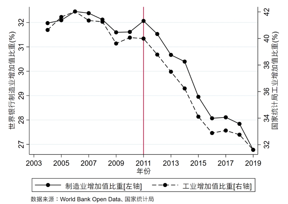
label var year "年份"
label var per "制造业增加值比重[左轴]"
label var tjj "工业增加值比重[右轴]"
graph twoway (connect per year ,yaxis(1) color(black) )   ///
(connect tjj year ,yaxis(2) color(black) lpattern(dash)  ) ///
, graphregion(color(white))  xlabel(2003(2)2019) ///
ytitle("世界银行制造业增加值比重(%)",axis(1) height(5))  ///
ytitle("国家统计局工业增加值比重(%)",axis(2) height(5))  ///
note(数据来源:World Bank Open Data、国家统计局) xline(2011)
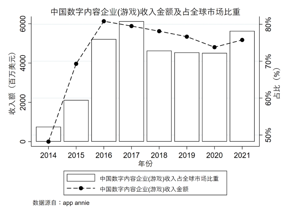
label var year "年份"

tw bar mR1 year,yaxis(2) bc(balck) sort barwidth(0.9) fintensity(inten0) ///
ylabel(0(2000)6000, axis(2)) ///
xlabel(2014(1)2021)|| ///
connect percent_R year,yaxis(1) lc(black) lp(dash) mc(blace) ///
ylabel(0.5 "50%" 0.6 "60%" 0.7 "70%" 0.8 "80%" ,axis(1))  ||, ///
graphregion(color(white) ) ///
bgcolor(white) ///
title("中国数字内容企业(游戏)收入金额及占全球市场比重", c(black) size(*0.8)) ///
ytitle("占比(%)",axis(1) height(7))  ///
ytitle("收入额(百万美元)",axis(2) height(5))  ///
legend(label(1 "中国数字内容企业(游戏)收入占全球市场比重") label(2 "中国数字内容企业(游戏)收入金额") ) ///
legend(size(small) col(1)) ///
note("数据源自:app annie")

graph save "Graph" "$path\output\playdata_1_percent_and_value_of_Chinese_Apps_Export.gph",replace
use hs_adj_year_PQV_2000_2015.dta,clear
use hs_adj_year_PQV_2000_2015_cregime10,clear
merge m:1 hs_adj using equipment
replace BEC=4 if BEC==1 & equipment!=1
destring hs_adj,replace
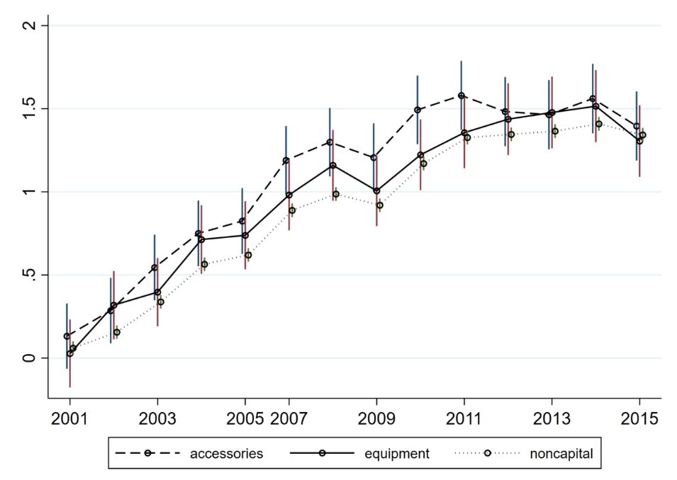
reghdfe lnV i.year if year!=2006 & BEC==2, a(hs)
est store result_accessories
reghdfe lnV i.year if year!=2006 & BEC==4, a(hs)
est store result_equipment
reghdfe lnV i.year if year!=2006 & BEC==0, a(hs)
est store result_noncapital
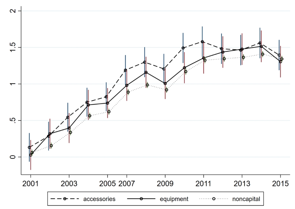
#d ;
coefplot
(result_accessories,c(l) label("accessories") lp(dash) lc(black) mc(black) ms(smcircle_hollow) offset(-0.07))
(result_equipment ,c(l) label("equipment") lp(solid) lc(black) mc(black) ms(smcircle_hollow))
(result_noncapital,c(l) label("noncapital") lp(dot) lc(black) mc(black) ms(smcircle_hollow) offset(0.07))
, vertical
drop(_cons) byopts(xrescale)
xlabel(1 "2001" 3"2003" 5"2005" 6"2007" 8"2009" 10"2011" 12"2013" 14"2015")
graphregion(color(white))
legend(size(small) col(3))
;
#d cr
主题设定
set scheme s2color    //  默认绘图主题
set scheme cleanplots, perm
set scheme plotplain, perm
set scheme plotplainblind , perm
set scheme burd, perm
set scheme tufte, perm
字体大小 option
| 字体大小option | description |
|---|---|
| zero | no size whatsoever, vanishingly small |
| minuscule | smallest |
| quarter_tiny | |
| third_tiny | |
| half_tiny | |
| tiny | |
| vsmall | |
| small | |
| medsmall | |
| medium | |
| medlarge | |
| large | |
| vlarge | |
| huge | |
| vhuge | largest |
| tenth | one-tenth the size of the graph |
| quarter | one-fourth the size of the graph |
| third | one-third the size of the graph |
| half | one-half the size of the graph |
| full | text the size of the graph |
| size | any size you want |
节点样式 eg: msymbol(O) mlcolor(gs5) mfcolor(gs12)
| symbolstyle | Synonym(if any) | Description | |
|---|---|---|---|
| circle | O | solid | |
| diamond | D | solid | |
| triangle | T | solid | |
| square | S | solid | |
| plus | + | ||
| X | X | ||
| arrowf | A | filled arrow head | |
| arrow | a | ||
| pipe | |||
| V | V | ||
| smcircle | o | solid | |
| smdiamond | d | solid | |
| smsquare | s | solid | |
| smtriangle | t | solid | |
| smplus | |||
| smx | x | ||
| smv | v | ||
| circle_hollow | Oh | hollow | |
| diamond_hollow | Dh | hollow | |
| triangle_hollow | Th | hollow | |
| square_hollow | Sh | hollow | |
| smcircle_hollow | oh | hollow | |
| smdiamond_hollow | dh | hollow | |
| smtriangle_hollow | th | hollow | |
| smsquare_hollow | sh | hollow | |
| point | p | a small dot | |
| none | i | a symbol that is invisible |
线样式
| linepatternstyle | Description |
|---|---|
| solid | solid line |
| dash | dashed line |
| dot | dotted line |
| dash_dot | |
| shortdash | |
| shortdash_dot | |
| longdash | |
| longdash_dot | |
| blank | invisible line |
| formula | e.g.,-. or –.. etc. |
| A formula is composed of any combination of | |
| l | solid line |
| _ | (underscore) a long dash |
| - | (hyphen) a medium dash |
| . | short dash (almost a dot) |
| # | small amount of blank space |
颜色
| black | edkblue | gs12 | lime | orange |
|---|---|---|---|---|
| blue | eggshell | gs13 | ltblue | orange_red |
| bluishgray | eltblue | gs14 | ltbluishgray | pink |
| bluishgray8 | eltgreen | gs15 | ltbluishgray8 | purple |
| brown | emerald | gs16 | ltkhaki | red |
| chocolate | emidblue | gs2 | magenta | sand |
| cranberry | erose | gs3 | maroon | sandb |
| cyan | forest_green | gs4 | midblue | sienna |
| dimgray | gold | gs5 | midgreen | stone |
| dkgreen | gray | gs6 | mint | sunflowerlime |
| dknavy | green | gs7 | navy | teal |
| dkorange | gs0 | gs8 | navy8 | white |
| ebblue | gs1 | gs9 | none | yellow |
| ebg | gs10 | khaki | olive | |
| edkbg | gs11 | lavender | olive_teal |
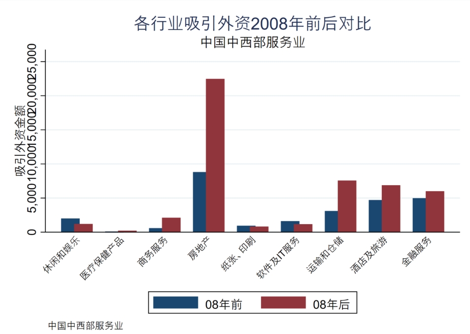
(2)柱状图
#delimit ;
graph bar cn_wzje_80 cn_wzje_81 if sec=="纸张、印刷", over(sec) bargap(-30)
  ytitle("吸引外资金额")
  legend( label(1 "08年前") label(2 "08年后") )
  title("吸引外资2008年前后对比")
  subtitle("纸张、印刷")
  graphregion(color(white))
  note("中国中西部服务业") ;
#delimit cr
graph bar (mean) percent1 (mean) percent1 , over(SNA) ///
nofill percentage stack  ///
bar(1, fcolor(gs1) lcolor(black) lwidth(thin)) ///
bar(2, fcolor(gs4) lcolor(black) lwidth(thin)) ///
bar(3, fcolor(gs7) lcolor(black) lwidth(thin)) ///
bar(4, fcolor(gs11) lcolor(black) lwidth(thin)) ///
bar(5, fcolor(gs13) lcolor(black) lwidth(thin)) ///
ytitle(Fraction of N_firm2 in $keepyear) ylabel(0(10)100, angle(horizontal)) ///
legend(order(1 "EU" 2 "JPN" 3 "KOR" 4 "USA" 5 "others") rows(1) ///
region(lcolor(white))) graphregion(fcolor(white)) plotregion(lcolor(black))
graph bar (sum) ActiveUsers1 ActiveUsers2 ActiveUsers3 , over(year) ///
	 stack bar(1, color(navy)) bar(2, color(khaki )) ///
	bar(3, color(gs6)) ylabel(,nogrid) 	///
	legend(label (1 "Southeast Asia") label (2 "Japan and South Korea") label (3 "Europe and America")) ///
	legend(size(small) col(3)) ///
	title("The scale of China's game App Active Users varies across different target countries",size(small))
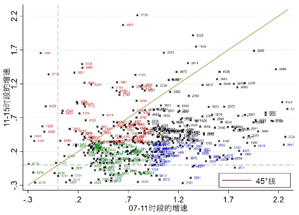
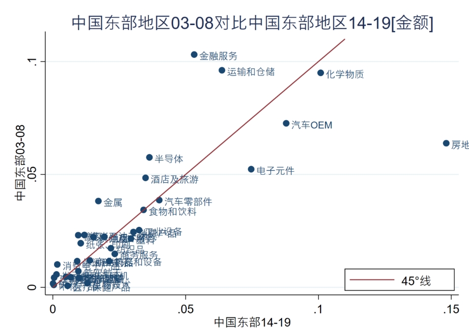
(3)散点图
graph twoway (scatter sc1 sc2 if wzlx_xf==1, mlabel(sec) mlabv(sec) ) (function y=x, range(-10000 10000)) , ///
title("高端制造业吸引外资   [09-14]较[03-08]变化值") ///
ytitle("中国中西部") ///
xtitle("东盟") ///
legend(ring(0) pos(5) order(2 "45°线")) ///
graphregion(color(white))
tw (scatter delta_v2_v3 delta_v1_v2 if delta_v1_v2>=-0.3& delta_v1_v2 <=2.3 ///
&delta_v2_v3>= -0.3&delta_v2_v3<=2.3, ///
mlabel(hy4) mlc(black) mlabc(black) ms(x) mlabs(tiny)) ///
(fun y=x,range(-0.3 2.3)) , ///
xlab(-0.3(0.5)2.3) ylab(-0.3(0.5)2.3)  ///
graphregion(color(white)) ///
xline(0,lp(dash) lc(gs10)) ///
yline(0,lp(dash) lc(gs10)) ///
legend(ring(0) pos(5) order(2 "45°线")) ///
ytitle("11-15时段的增速") ///
xtitle("07-11时段的增速")
graph twoway (scatter c_AS c_WD, mlabel(cic03)  ) (lfit c_AS c_WD) , ///
title("东盟增速放缓 vs 世界增速放缓")  ///
ytitle("东盟")  ///
xtitle("世界") ///
legend(ring(0) pos(5) order(2 "拟合")) ///
graphregion(color(white))
tw (scatter percent1 percent2 if develop_IMF == 1 ,mlab(iso_ded) mlabsize(vsmall) ms(oh)) ///
(scatter percent1 percent2 if develop_IMF == 0 , mlabsize(vsmall) mc(red) ms(oh)) ///
(fun y=x, range(0 0.003)), ///
ytitle("00-06年进口占比(%)",axis(1) height(5)) ///
xtitle("11-05年进口占比(%)",axis(1) height(5)) legend(off)
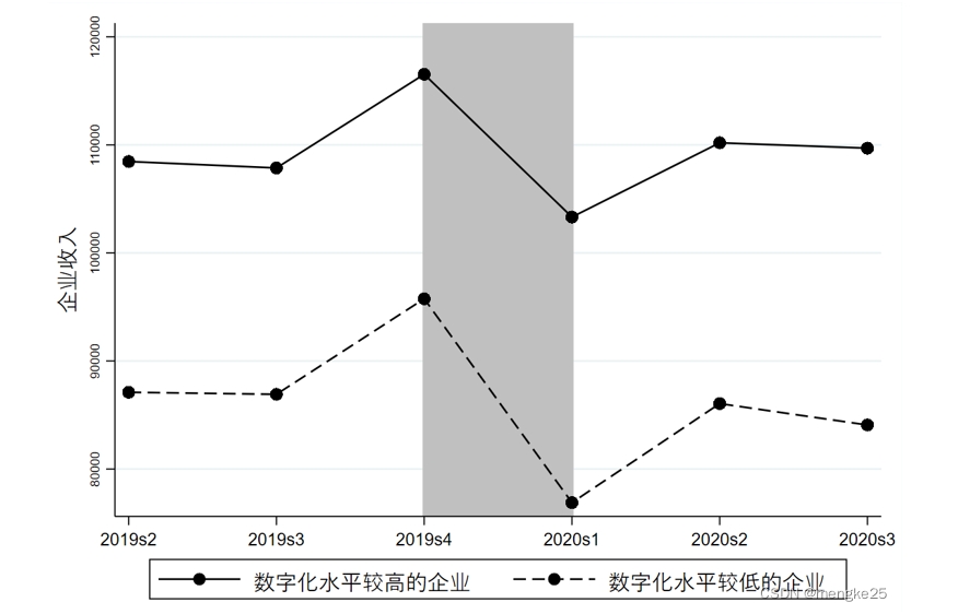
(4)bgshade
bgshade ks, shaders(uu9)  ///
   twoway(connect lamda22 ks if treat==1&ks>=6&ks<=11 ||             ///
          connect lamda22 ks if treat==0&ks>=6&ks<=11 , xlab(6(1)11) ///
   title("新冠疫情冲击下企业平均收入变化趋势"))
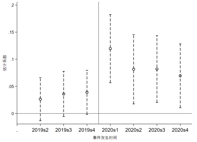
(5)coefplot
coefplot,  levels(90) vertical lcolor(black)mcolor(black) ///
 msymbol(circle_hollow) ytitle(估计系数, size(small)) ///
 ylabel(, labsize(small) angle(horizontal) nogrid) ///
 yline(0, lwidth(vthin)lpattern(solid) lcolor(black)) ///
 xtitle(事件发生时间, size(small)) ///
  title("(B)企业缴税的平行趋势检验") ///
 xlabel(0"." 1"2019s2" 2"2019s3" 3"2019s4" 4"2020s1" 5"2020s2" 6"2020s3" 7"2020s4")
reghdfe lnQ i.Year if elec == 1,a(i.citycode) vce(r)
est store elec_Q_1

reghdfe lnV i.Year if elec == 1,a(i.citycode) vce(r)
est store elec_V_1


reghdfe lnQ i.Year if elec == 0,a(i.citycode) vce(r)
est store elec_Q_0

reghdfe lnV i.Year if elec == 0,a(i.citycode) vce(r)
est store elec_V_0

coefplot (elec_Q_1,label("半导体电子元件相关企业进口数量") offset(0.05)  pstyle(p3)) ///
(elec_Q_0 ,label("非半导体电子元件相关企业进口数量") offset(-0.05)  pstyle(p4) ), ///
vertical drop(_cons) xline(0) ///
graphregion(color(white)) ///
yline(0) ///
addplot(line @b @at,lp(dash) lwidth(*0.5)) ///
legend(label(1 "半导体电子元件相关企业进口数量") label(2 "非半导体电子元件相关企业进口数量") )
#d ;
coefplot
  (low_sna1,c(l) label("") lp(solid) lc(red) mc(red) ms(smcircle_hollow) offset(-0.06) noci)
  (low_sna23,c(l) label("") lp(dash) lc(black) mc(black) ms(smcircle) offset(-0.02) noci)
  , vertical
  drop(_cons  meanfre lnT) byopts(xrescale)
  graphregion(color(white))
  legend(size(small) col(3))
  yline(0 ,lc(navy) lp(dash_dot))  level(95)
  xlabel(, ang(45) labsize(vsmall)) c(l)
  title(`v',size(small))
  legend(off)
  ;
#d cr
(6)画系数和置信区间
twoway (scatter coef week) ///
(rcap ci_lower ci_upper week, ///
 lcolor(black) ///
 mcolor(black) ///
 lwidth(vthin) ///
 lpattern(dash) ///
 msymbol(circle_hollow) ///
 legend(label(2 "99% CI"))) , ///
yline(0) ///
xtitle("")  ///
graphregion(fcolor(white)) ///
title("第X周的系数", size(medium)) ///
name("Coef_all_I", replace)
(7)画直方图
hist year if year>=1400 & year<=2010, freq bin(200) ylabel(0(500)2500) xtitle("Year") xline(1950 1980,lw(thin)) ///
     text(1500 1950 "Year=1950", place(w)) text(2000 1980 "Year=1980", place(w))
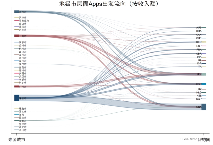
(8)画桑基图
cd $path\appdata
use Data_games.dta,clear
merge m:1 ParentCompanyName using "$path\data\company_city"
keep if _m == 3
drop _m
gen from = city_code
encode iso3_j,gen(to)
bys from to :egen tR = total(Revenue)
bys from to :egen tD = total(Downloads)
duplicates drop  from to ,force
gen x0 = 1
gen x1 = 2
tostring city_code ,gen(city2)
drop if dest == "CHN"

sankey_plot x0 from x1 to, ///
width0(tR) extra xlabel(1 "Source" 2 "Destination", nogrid labsize(small)) ///
colorpalette(economist, opacity(30)) ///
label0(city) label1(iso3_j) ///
labsize(*0.6) labcolor(black) ///
graphregion(color(white))  gap(0.1) ///
title("地级市层面Apps出海流向(按收入额)",color(black) size(*0.8))

graph save "Graph" "$path\output\sankey_R_0228.gph",replace


sankey_plot x0 from x1 to, ///
width0(tD) extra xlabel(1 "Source" 2 "Destination", nogrid labsize(small)) ///
colorpalette(economist, opacity(30)) ///
label0(city) label1(iso3_j) ///
labsize(*0.6) labcolor(black) ///
graphregion(color(white))  gap(0.1) ///
title("地级市层面Apps出海流向(按下载量)",color(black) size(*0.8))

graph save "Graph" "$path\output\sankey_D_0228.gph",replace
(9)分组看分布——hbox和vioplot
reghdfe lnexp i.hy2 ,noa vce(r)
predict e
ren e e1
gen ex = lnexp - e1

graph hbox ex, ///
over(hy2_name)  ///
ylabel(, labsize(tiny) ) ///
title("不同行业离散程度(通过残差反映)", c(black) size(*0.8))

vioplot ex, over(hy2_name) horizontal name(myplot2) ///
   title("不同行业离散程度(通过残差反映)") ///
   ytitle(行业) ///
   ylab(, angle(horiz))
(10)分组看分布——hbox和vioplot
vioplot year if Affiliates == 0, ///
over(N_iso3j) vertical subtitle("",size(small)) ytitle(Year) ///
xtitle("Num. of New destination") ylab(, angle(horiz)) ///
yline(2018,lc(red) lp(dash)) xline(14.5,lc(red) lp(dash)) ///
subtitle("Domestic",size(small)) //name("fig1")

vioplot year if Affiliates == 1, ///
over(N_iso3j) vertical subtitle("",size(small)) ytitle(Year) ///
xtitle("Num. of New destination") ylab(, angle(horiz)) ///
yline(2018,lc(red) lp(dash)) xline(14.5,lc(red) lp(dash)) ///
subtitle("Affiliates",size(small)) //name("fig2")

graph combine fig1 fig2 ,col(2) row(1) iscale(1) xsize(20) ysize(10)
(11)堆叠的区域阴影增长趋势
tw (rarea tv v1 year,fcolor(gs5)) ///
   (rarea v1 xx year,fcolor(gs10)) , ///
   legend(col(2) label (1 "Export")  ///
          label (2 "Import")) ///
   xlabel(2003(2)2021) ///
   ylabel(,nogrid) ///
   xtitle("Years") ///
   ytitle("Trade Value (in million USD)") ///
   name(fig1_2,replace)
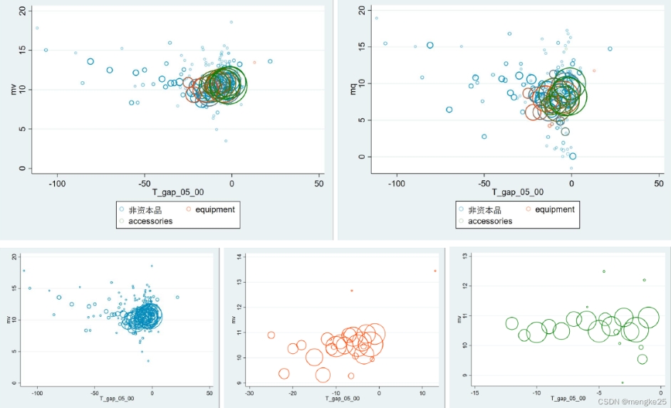
(12)气泡图
twoway(scatter mv T_gap_05_00 [fweight=N] if BEC == 0&T_gap_05_00!=0&N !=0,msymbol(Oh) mc(ebblue%40)) ///
(scatter mv T_gap_05_00 [fweight=N] if BEC == 4&T_gap_05_00!=0&N !=0,msymbol(Oh) mc(orange_red%40)) ///
(scatter mv T_gap_05_00 [fweight=N] if BEC == 2&T_gap_05_00!=0&N !=0,msymbol(Oh) mc(green%20)) ///
, legend(label(1 "非资本品") label(2 "equipment") label(3 "accessories") )
2. 处理数据
(1)拓展expand数据
| freq | count | value |
|---|---|---|
| 1 | 9523 | 4845.1143 |
| 2 | 9524 | 969.66498 |
| 2 | 9525 | 129.53349 |
| 2 | 9526 | 71284.508 |
| 2 | 9527 | 1038.127 |
| 2 | 9528 | 445877.09 |
count是id的唯一识别码,expandcl函数可以生成freq行相同的样本,并生成一个新的id识别码freq_count
egen count=group(id hs02_6)
expandcl freq,gen(freq_count) cluster(count)
drop freq_count
(2)时间数据
gen R= mdy(month_r,day_r,year_r)
gen week_r = week(R)
gen day_r = day(R)
gen dow_r = dow(R)  //返回周几
gen doy_r = doy(R)  //返回年内日期
gen yw_r = yw(year_r,week_r)
gen ed = yw - yw_r
//yw ym yq yh分别为年周、年月、年季、年半年
gen period_kb= date(date_u,"YMD")-date(date_kb,"YMD")
(3)常见函数
int(x) //取整,不论后面的小数是什么,只取小数点前的数值
round(x) // 四舍五入取整
round(x, .01) //保留两位小数四舍五入
gen y = sum(x)  //求列累积和
egen y = sum(x) //求列总和
egen y = rsum(x y z) //求x+y+z总和
egen y = rowmean(x y z) //求(x+y+z)/3
egen y = rowsd(x y z) //求x y z的方差
egen y = rowmim(x y z) //求x y z的最小值
egen y = rowmax(x y z) //求x y z的最大值
egen y = mean(x)      //求列均值
egen y = median(x)    //求列中位数
egen y = std(x)       //求变异系数,与方差不同

bysort x(y): gen z = y[1] //按照x分组,分组后按照y排序,生成一个新变量z=y的第一个观察值
(4)缩尾处理
foreach v of var DexpoAS4- DlnexpoWD2{
gen `v'_w=`v'
qui su `v',det
replace `v'_w=r(p99) if `v'>r(p99) & `v'<.
replace `v'_w=r(p1) if `v'<r(p1)
}

winsor2 wage, replace cuts(1 99) trim
summary 一个变量之后,可以返回的结果有
r(N)           //number of observations
r(mean)        //mean
r(skewness)    //skewness (detail only)
r(min)         //minimum
r(max)         //maximum
r(sum_w)       //sum of the weights
r(p1)          //1st percentile (detail only)
r(p5)          //5th percentile (detail only)
r(p10)         //10th percentile (detail only)
r(p25)         //25th percentile (detail only)
r(p50)         //50th percentile (detail only)
r(p75)         //75th percentile (detail only)
r(p90)         //90th percentile (detail only)
r(p95)         //95th percentile (detail only)
r(p99)         //99th percentile (detail only)
r(Var)         //variance
r(kurtosis)    //kurtosis (detail only)
r(sum)         //sum of variable
r(sd)          //standard deviation
(5)创建文件夹
efolder, cd(D:\stata15\hxs\连享会007)
efolder, cd(D:\stata15\hxs\连享会007) sub(侯新烁 连玉君 007小组1号成员 007小组2号成员)
(6)bysort的替代方案
*展示根据highzupu50(族谱)和year分组后的变量drqianfen(死亡率)均值;
collapse (mean) drqianfen, by(highzupu50 year)
(7)定义无缺失的样本
g rsample = !mi(avggrain_fyr) & !mi(nograin_fyr) & !mi(urban_fyr)& !mi(dis_bj_fyr) & !mi(dis_pc_fyr) & !mi(migrants_fyr)& !mi(rice_fyr) & !mi(minor_fyr) & !mi(edu_fyr)
(8)定义Dummy的新替代式(时间range)
*如果yob满足1825≤yob≤1899则pre取值为1,否则pre取值为0。mid、post生成过程类似。
gen pre = inrange(yob, 1825, 1899)
gen mid = inrange(yob, 1899, 1919)
gen post = inrange(yob, 1920, 1960)
(9)快速替换
recode treatyear (1969 = 1) (1979 = 2) (1989 = 3) (1999 = 4) (2009 = 5)
3. 处理字符
(1)替换字符
replace 候选人姓名=subinstr( 候选人姓名, " ", "",. )
(2)捕捉字符中的某些特征
keep if strmatch(city, "*山东*")
gen temp = 1 if strmatch(reporteriso3, "A*")
(3)提取字符,检索特定字符
//从enddate字符1开始取,取4个字符赋给year
gen year = substr(enddate,1,4)

//strpos(s1, s2)返回字符s2在s1中的位置,如果s1中找不到s2,则返回0,将该判断再赋给y
gen y = strpos(s1, s2) != 0
4. 输出结果
(1)常规输出
outreg2 using "E:\mfg\outreg\r2", word append addtext(CountryFE, YES,YearFE, YES)
(2)iv回归输出第一阶段
eststo: xtivreg p_a_w (DexpoCN4_w=dexpo44) ///
 i.t c.expr0#t c.Lshare0#t ///
 c.lnGDP0#t c.lngdp0#t, fe first vce(cluster c)

 eststo: xtreg DexpoCN4_w dexpo44 ///
 i.t c.expr0#t c.Lshare0#t ///
 c.lnGDP0#t c.lngdp0#t if e(sample)==1 ,fe
 cd $path\outreg
 outreg2 using "table3", word replace addtext(CityFE, YES,YearFE, YES) keep(dexpo44)
(3)变量描述性统计
*列出inv等变量的样本数、均值、标准差、最小值和最大值。
tabstat inv loginv log_levies ///
     logpopl logincome logasset hhsize landpc logmigration logtax logtransfer share_admin  ///
	 postcont postopen secret_ballot proxy_voting moving_ballot ///
	 , s(N mean sd min max) c(s)
logout,save(summary) word replace:tabstat lnActiveUsers lnDownloads per_mws lnGDP0 lngdp0 lnpopu_RD0 lnper_ind30 lnpopu_ind30 lnpopu_ict0,s(N mean sd min max) f(%12.3f) c(s)
(4)est store以及esttab输出结果
reghdfe Y1 did ,a(i.city_code i.t#i.ison_j)  vce(r)
est store fit1

reghdfe Y1 did $basecontrols1 ,a(i.city_code i.t#i.ison_j) vce(r)
est store fit2

reghdfe Y2 did ,a(i.city_code i.t#i.ison_j)  vce(r)
est store fit3

reghdfe Y2 did $basecontrols1 ,a(i.city_code i.t#i.ison_j) vce(r)
est store fit4

estfe fit1 fit2 fit3 fit4, labels(i1.city_code "cityFE"  t#ison_j "Time-CountryFE")
esttab fit1 fit2 fit3 fit4, mtitle("收入" "收入" "下载量" "下载量") b(%6.4f) p(%6.2f) scalar(N F r2_a) indicate(`r(indicate_fe)')
5.矩阵保存结果
mat T1 = J(3,3,.)

reghdfe temp ib1.season if year == 2018 & treat == 1,noa
forvalues i = 1/3{
	local j = `i' + 1
	mat T1[`i',1] = _b[`j'.season]
}

reghdfe temp ib1.season if year == 2019 & treat == 1,noa
forvalues i = 1/3{
	local j = `i' + 1
	mat T1[`i',2] = _b[`j'.season]
}

reghdfe temp ib1.season if year == 2020 & treat == 1,noa
forvalues i = 1/3{
	mat T1[`i',3] = _b[`=1+`i''.season]
}


svmat T1
6.导入数据(全字符串)
forv i = 2000/2003{
	cd E:\Data\EPS工企海关匹配库\origindata
	import delimited "工企+海关(`i').csv", stringcols(_all) clear
	cd E:\Data\EPS工企海关匹配库
	save data`i'.dta,replace
}
7.循环
clear all
set obs 1000
**#** 用forvalues循环对单一变量进行处理
gen id = .
//生成一个变量名为id,代表第几个人,假设一共有50个人
//假设每个人都有20个观测值,代表20年
forvalues i = 1/50 {
local j = `i' - 1 //暂时定义0~49 方便计算
local lower = `j' * 20 +1 //定义下限 1、21、41、61
local upper = `j' * 20 + 20 //定义上限 20、40、60、80
//由此就定义了 1~20 21~40 41~60 ……
replace id = `i' in `lower'/`upper' //给第1~20行,赋值为第1个人
//给第21~40行,赋值为第2个人
}
bys id : gen T = _n + 2000 //对于每个人,都生成一个时间序列
**#** 用forvalues循环对多个变量进行处理
forvalues i = 1/5 {
gen value`i' = .
cap gen e = rnormal()
replace value`i' = e * 10 + `i'
cap drop e
}
// 等价于
gen value6 = .
cap gen e = rnormal()
replace value6 = e * 10 + 6
cap drop e
gen value7 = .
cap gen e = rnormal()
replace value7 = e * 10 + 7
cap drop e
gen value8 = .
cap gen e = rnormal()
replace value8 = e * 10 + 8
cap drop e
gen value9 = .
cap gen e = rnormal()
replace value9 = e * 10 + 9
cap drop e
gen value10 = .
cap gen e = rnormal()
replace value10 = e * 10 + 10
cap drop e
**#** 用while循环对单一变量进行处理
// 只要时间在T=11和T=20之间,就对value1~value10进行 " 乘0.1"的处理
local i = 2010
while `i' < 2020 {
forvalues j = 1/10{
replace value`j' = value`j' * 0.1 if T == `i'
}
local i = `i' + 1
}
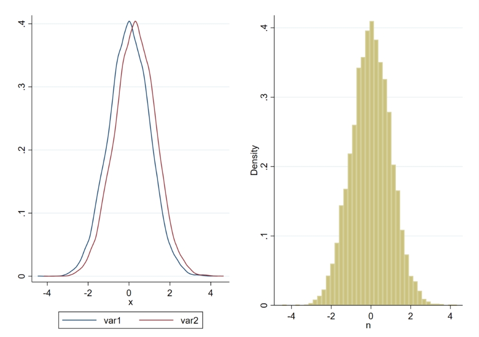
**#** 用foreach对变量进行处理
foreach v in value1 value2 value3 value4 value5 {
su `v' ,d
replace `v' = (`v' - r(min)) / (r(max) - r(min))
kdensity `v'
}
// 等价于
su value6,d
replace value6 = (value6 - r(min)) / (r(max) - r(min))
kdensity value6
su value7,d
replace value7 = (value7 - r(min)) / (r(max) - r(min))
kdensity value7
su value8,d
replace value8 = (value8 - r(min)) / (r(max) - r(min))
kdensity value8
su value9,d
replace value9 = (value9 - r(min)) / (r(max) - r(min))
kdensity value9
su value10,d
replace value10 = (value10 - r(min)) / (r(max) - r(min))
kdensity value10
8.循环数字-标注“文字”
cd $path_EPS_data
use temp_ybmy_nodest.dta,clear
gen hy3 = real(substr(string(hy4),1,3))
gen hy2 = real(substr(string(hy4),1,2))

gen lnv = ln(1+v)
gen lnq = ln(1+q)

merge m:1 hy2 using "$path_local_data\cic_hy2_Chinese_name.dta"
drop _m

preserve
keep hy2*
duplicates drop hy2,force
global length = _N
forv i = 1/$length {
	local j = hy2 in `i'
	su hy2 in `i',d
	sca int`j' = r(mean)
	sca s`j' = hy2_name in `i'
}
restore

capture{
forv i = 13/45{
    reghdfe lnv i.year if hy2 == `i', noa vce(r)
	eststo fit`i'
}
}

capture{
forv i = 13/45{
local hy = int`i'
local gamma = s`i'
#d ;
coefplot
  (fit`i',c(l) label(`hy':`gamma') lp(dash) lc(black) mc(black) ms(smcircle_hollow) offset(-0.07))
  , vertical
  drop(_cons) byopts(xrescale)
  xlabel(1 "2008"  2"2009"  3"2010" 4"2011" 5"2012" 6"2013" 7"2014" 8"2015")
  graphregion(color(white))
  legend(size(small) col(3))
  ;
#d cr
graph export "$path_output\hy`i'_`gamma'.png", as(png) name("Graph") replace
}
}
9.拟合选项
| fit情况 |
|---|
| [G-2] graph twoway line — Twoway line plots |
| [G-2] graph twoway qfit — Twoway quadratic prediction plots |
| [G-2] graph twoway fpfit — Twoway fractional-polynomial prediction plots |
| [G-2] graph twoway mband — Twoway median-band plots |
| [G-2] graph twoway mspline — Twoway median-spline plots |
| [G-2] graph twoway lfitci — Twoway linear prediction plots with CIs |
10.工具变量第一阶段
不可识别统计量是Klei-Paap 弱识别统计量是Cragg-Donald 工具变量外生是Hansen-J
前两个是得拒绝原假设,最后一个是得接受原假设
11.国民经济行业分类
// 大类代码reshape后加labe
label var Nfirm_ind1 "农、林、牧、渔业"
label var Nfirm_ind2 "采矿业"
label var Nfirm_ind3 "制造业"
label var Nfirm_ind4 "电力、热力、燃气及水生产和供应业"
label var Nfirm_ind5 "建筑业"
label var Nfirm_ind6 "批发和零售业"
label var Nfirm_ind7 "交通运输、仓储和邮政业"
label var Nfirm_ind8 "住宿和餐饮业"
label var Nfirm_ind9 "信息传输、软件和信息技术服务业"
label var Nfirm_ind10 "金融业"
label var Nfirm_ind11 "房地产业"
label var Nfirm_ind12 "租赁和商务服务业"
label var Nfirm_ind13 "科学研究和技术服务业"
label var Nfirm_ind14 "水利、环境和公共设施管理业"
label var Nfirm_ind15 "居民服务、修理和其他服务业"
label var Nfirm_ind16 "教育"
label var Nfirm_ind17 "卫生和社会工作"
label var Nfirm_ind18 "文化、体育和娱乐业"
label var Nfirm_ind19 "公共管理、社会保障和社会组织"
label var Nfirm_ind20 "国际组织"
12.egen 函数
| 函数 | 用法 | 释义 |
|---|---|---|
| xtile | egen A = xtile(n) ,nq(10) | 对于n变量生成分位数,分位数的范围用nq=10来度量 |
| corr | egen B = corr(temp1 temp2) | 对于temp1和temp2变量生成相关系数 |
| ereplace | 对标egen,能够替换原变量 | |
| clsst | egen ii = clsst(n) , v(1(1)10) | 给n变量按照从小到大的次序赋以v值 |
| base | egen ii = base(n) | 给n变量生成一个二进制字符串变量ii |
| msub | egen newstr = msub(strvar), f(A B C) r(1 2 3) | replaces “A” by “1”, “B” by “2”, “C” by “3” |
| egen newstr = msub(strvar), f(`”””’) | deletes quotation mark “ | |
| egen newstr = msub(strvar) f(frog) w | deletes “frog” only if occurring as single word | |
| ntos | egen grade = ntos(Grade), from(1/5) to(Poor Fair Good “Very good” Excellent) | 给Grade变量生成字符串 |
| repeat | egen quarter = repeat(), v(1/4) | 生成一个quarter变量,重复1-4 |
| egen quarter = repeat(), v(1/4) block(3) | 生成一个quarter变量,重复1-4,其中1重复3次,2重复3次,3重复3次 | |
| adju | bys id : egen nu = adju(n) | 生成一个新变量nu等于n的upper值 |
| adjl | bys id : egen nl = adjl(n) | 生成一个新变量nu等于n的lower值 |
| gmean | egen gmean = gmean(mpg), by(rep78) | geometric mean |
| hmean | egen hmean = hmean(mpg), by(rep78) | harmonic mean |
| outside | bys id : egen dd = outside(n) | 找到n的极端值,并赋值给dd |
| ridit | bys id : egen dr = ridit(n) | 近似于分位数,relative to identified distribution unit |
| sumoth | bys id : egen xrd = sumoth(n) | 加总本组内除了自身之外的其他数值 |
| pctile | bys id : egen p25 = pctile(n) ,p(25) | 求分位数 |